Hooked on Uniswap

A paper written with David Chang, Xincheng Zhang, and Nathan Wangidjaja for Science of Blockchains, taught by Tim Roughgarden.

1. Introduction

Uniswap was first launched in November 2018 as a new form of decentralized exchange. In contrast to previous decentralized exchanges (DEXs), Uniswap used an automated market maker (AMM) for determining exchange rates between different tokens. This feature is what truly made Uniswap stand out, as it significantly reduced the friction experienced by all parties when making a trade. Previous decentralized exchanges based on order books required active input from users to place orders, had delays before orders were fulfilled, and suffered from poor liquidity. Uniswap, however, calculated prices automatically. It also allowed anyone to make exchanges or provide liquidity without much complexity. Add on the fact that its solution could be elegantly summed up as "x*y=k", Uniswap quickly took off, paving the way for massive innovations in DEXs during the years to come. There have been 4 separate versions of Uniswap as of today, with V4 having been released in January 2025.

2. Uniswap V1 and Uniswap V2

2.1 Uniswap V1

Uniswap V1's main innovation was its new AMM and "x·y=k" formula for price calculation. In general terms, the amount of one token in a liquidity pool, x, multiplied by the amount of the other token, y, should be equal to a constant. Intuitively, this means that the more scarce a token is, the more valuable it gets. The larger the x/y ratio, the more someone would have to pay in y to get a fixed amount of x. If we're trading some of token X for token Y, this may generally be represented by the equation below,

Variations of this equation can be used to determine for a fixed output amount Δy, how much input Δx a user needs [1]. Or for a fixed input Δx, how much output Δy a user can get back. This formulation is useful because it allows for trading to happen no matter the amount of each token in a pool, and prevents the pool from ever running out of liquidity. In fact, not only did the Uniswap AMM enable continuous liquidity, but it also caused the ratio of the two tokens amounts to tend toward their actual market exchange rate.

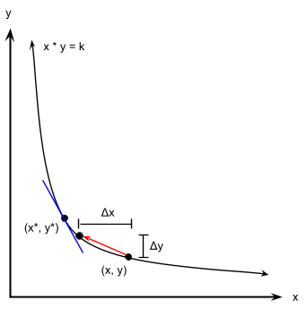
One way to think about this is to consider the visualization below. In the graph, the x-axis indicates the amount of token X and the y-axis indicates the amount of token Y in a liquidity pool. (x*, y*) indicates the point where the amounts in the liquidity pool are such that the exchange rate equals the actual market exchange rate of the two tokens. Notice the blue line, which is the slope of the curve at point (x*, y*). This indicates the exchange rate at point (x*, y*), i.e. if one were to exchange a tiny amount of x or a tiny amount of y. Because of the x·y=k formulation, the slope of the blue line is exactly equal to the ratio y*/x*.

Now if the actual amount of each token was at the point (x, y) on the curve, someone could make money by trading some of token X for some of token Y. If they were to put up Δx of token X they would move the point (x, y) up along the curve to a point (x − Δx, y + Δy), where Δy is determined by the curve and how much we move the x-coordinate (Δx). Doing so would allow them to trade Δx of X tokens for Δy of Y tokens. This ratio Δx/Δy depends on Δx and the actual curve, but one example is shown using the red arrow. Notice that Δx/Δy is always better than x*/y* when (x, y) is to the right side of the curve from (x*, y*). Similarly if (x, y) were on the left side of the curve from (x*, y*) then someone could trade token Y for token X at a rate Δy/Δx strictly better than y*/x*.

So if the current exchange rate didn't match the market exchange rate, people were incentivized to bring it back to the market rate and make a profit.

This is the general concept of x·y=k, but the formulation is actually more complex due to factoring in a base 0.3% fee associated with any exchange on a liquidity pool. This fee is such that whenever someone wishes to exchange tokens and puts in a certain amount, only 99.7% of the amount they put in is used in calculating how much of the other token they get back. In other words, the equation actually used by V1's AMM is the following:

The 0.003 · Δx gets added to the pool for free, and is not included in the constant product calculation. In Uniswap V1, liquidity providers are rewarded via trading fees, which increase the total reserves in the pool over time. Although the product x·y remains approximately constant during each trade, the fees cause a net gain in pool value, benefiting LPs.

Making use of its AMM technology, Uniswap V1 offers two basic functionalities for users: liquidity providing and token exchanging. It enables this because it is a set of smart contracts on the Ethereum blockchain, written in the Vyper programming language. Its contracts include exchange contracts, each of which control the liquidity pool between ETH and an ERC-20 token. They have functions for users to provide liquidity to the pool and functions for users to exchange their tokens. These exchange contracts all follow a standard template. V1 also has what it calls a factory contract, which is used to keep track of all the exchange contracts that currently exist, as well as provide functionality for creating new ones [19].

For Uniswap's first functionality, exchanging tokens, Uniswap offers exchanges between ETH and any ERC-20 token. An ERC-20 token can be thought of as both a cryptocurrency as well as a smart contract on the Ethereum blockchain. A normal smart contract on the Ethereum blockchain is just a program with functions that can be called by users or other contracts on the Ethereum network. However, a contract for an ERC-20 token has a more specific, standardized interface designed for cryptocurrencies. It consists of features like a ledger mapping account addresses to how much of the token they own, as well as standard functions for transferring and receiving funds [19]. All in all, this means that Uniswap exchange contracts tend to interact directly with ERC-20 contracts when a user requests exchanges to be made.

The second core function of Uniswap V1 is liquidity provision. To participate, users must deposit ETH and an ERC-20 token in proportion to the current pool ratio. In return, they receive liquidity tokens representing their share of the pool. The proportion of tokens a user contributes determines the proportion of liquidity tokens they receive, relative to the total supply. These liquidity tokens can later be redeemed—burned—in exchange for the same share of the pool's ETH and ERC-20 reserves. While this mechanism formed a strong foundation for V1, it also set the stage for the more advanced features introduced in later versions of Uniswap.

2.2 Uniswap V2

Uniswap V2, released in May 2020, added some key features that improved the functionality of V1. Most notably, it included liquidity pools between any two ERC-20 tokens (rather than just ETH–ERC-20 pools). Aside from that, V2 provided additional support for using Uniswap as a price oracle and performing flash swaps.

To make all of these features possible, Uniswap V2 started with an overhaul of the software architecture used in V1. In V1, Uniswap consisted of two types of contracts written in Vyper: factory and exchange contracts. Users would interact with the factory contracts directly to create new ETH–ERC-20 liquidity pools, while they would interact with the exchange contract for a liquidity pool in order to do things like provide liquidity or exchange tokens.

In V2, this functionality is effectively split between a set of "core" contracts and a set of "periphery" contracts. "Core" contracts are extremely simple, and provide only the most basic, low-level functionalities required to store and access the resources of a particular liquidity pool. They are designed like this in order to guarantee the security of the tokens provided by liquidity providers, and are not intended to be called upon directly by users. Instead, users interact with the set of "periphery" contracts provided by Uniswap, which serve as a more high-level wrapper of the "core" contracts [20].

More explicitly, V2's core consists of a factory and a pair contract. The factory contract serves the same purpose of V1's factory contract, while the pair contract is analogous to V1's exchange contract. The difference is that the pair contract is designed to work with two ERC-20 tokens, rather than one ERC-20 token and ETH. In fact, for ETH–ERC-20 pools, ETH is wrapped into WETH so that the pair contract can interact with it the same way it would an ERC-20 token. Additionally, each pair contract now only contains functionality for adding/removing liquidity, and swapping some amount of one token for some amount of another. Checking the correct price of each swap falls to contracts in V2's periphery [20]. This periphery consists mainly of the router contract, which is used to reroute user actions to the correct core pair contracts, and the library contract, which contains useful helper functions such as determining the exchange rate between two tokens.

The first new feature of Uniswap V2 enabled by its re-architecture is ERC-20 to ERC-20 exchanges. Not only does this just provide more flexibility for users, allowing them to exchange directly for their desired tokens, but it also comes with a few practical considerations. Chief among these is the idea of impermanent loss for liquidity providers. Because the price of ETH can fluctuate a lot over time, whenever it does the ratio of reserves in a liquidity pool will no longer match the correct market exchange rate [21]. Thus, people can take advantage of this to make money by trading in the liquidity pool and exchanging tokens to bring the ratio of reserves back to the new market exchange rate. Each time this happens liquidity providers may suffer a loss in the sense that if they held onto their original tokens without putting them into the liquidity pool, they would have earned more profit.

To see this, consider an example where liquidity reserves consist of 1 ETH and 100 DAI (stablecoin that maintains close to a 1:1 exchange ratio with USD) at the current market exchange rate. If the exchange rate shifts to 1 ETH to 400 DAI, people will trade with the liquidity reserves until they reach 0.5 ETH / 200 DAI. If the original 1 ETH / 100 DAI was extracted from the pool and held onto instead, its value would have reached 500 DAI, but as of now the value of the pool is only 400 DAI plus the 0.3% fee from trades. If, for example, liquidity was provided in a pool between two stablecoins instead of ETH, however, there would be no significant fluctuations in price, and the liquidity providers would be able to make their 0.3% fee with significantly less risk of impermanent loss [21].

A second feature enabled by Uniswap V2 is oracle price calculations. Mainly, during the era of Uniswap V1, we saw that the ratio of a particular token with ETH in a liquidity pool had the property that it tended towards the market exchange rate due to the x·y=k constant product formula. Uniswap could therefore potentially be used as a source, or oracle to determine the current market exchange rate of ETH/token X on the ethereum mainnet. In other words, smart contracts that make use of this exchange rate information could potentially call Uniswap in order to get this information.

The main problem with using the V1 implementation as a price oracle directly however, was the fact that its price could easily be manipulated. Someone could simply make exchanges on a liquidity pool to shift prices in the direction they wanted and then run some transactions on the other contracts relying on the now falsified price information. Afterwards they could then simply trade back the tokens they traded to return the liquidity pool to its correct exchange rate.

To prevent this, a liquidity pool of Uniswap V2 calculates price by taking the ratio of its reserves at the start of every block in the Ethereum block chain, before the first transaction of the block is executed [2]. This means that someone trying to manipulate the price would have to target their manipulation towards the very end of a block, but if they are a bit off someone else could easily snatch the arbitrage opportunity, shifting the price back to the correct one before the end of the block. A miner with the ability to order transactions could still try to manipulate the price, but they would not be easily able to capitalize on it, because that would require them to also mine the next block.

However, if an attacker does somehow manage to pull off an attack like this, they could still stand to earn a significant profit that outweighs the cost required to do it. As another safety measure, Uniswap V2 provides a method for calculating the time-weighted average price (TWAP) [2]. This is done in Uniswap's core contracts by maintaining a cumulative sum variable in the contract for every pair. When it gets the price at the end of each block, the price multiplied by the time since the last block is added to the cumulative sum. In other words, the cumulative sum should approximately be the sum of all prices for every second the pool existed.

Where p_i is the price at time i (in seconds). Using this formulation, an external contract can calculate the TWAP or average price from times t1 to t2 by getting the cumulative sum at both t1 and t2. Then by subtracting those cumulative sums they would obtain the desired average.

This average price is far more resistant to attackers, since they would have to spend much more to control multiple price checks at the end of multiple blocks. External contracts using the V2 price oracle could also control t1 and t2. A larger window (t2 − t1) means a price more resistant to attackers, while a smaller window would mean a more up-to-date price.

A final feature included by V2 is flash swaps, which allow users to receive and use an asset before they actually pay for it. This works as long as the user is able to make use of the asset and provide payment for it within the same atomic transaction. V2 implements this feature specifically by transferring the tokens a user would receive from a swap immediately, and then running a callable function the user passes into the same swap function [2]. For example, a user can initiate a swap of x amount of token X for y amount of token Y. V2 then optimistically transfers y of token Y to the user's balances and runs their callable. After it is run, the user must return the token Y they "borrowed" or provide the token X needed for the swap. This requirement is such that a combination of token Y and token X may also be returned, as long as the product of the new reserves is greater than or equal to the product of the old reserves after fees. More explicitly,

A 0.3% fee is taken from any value x_in, y_in, the user uses to pay for the swap.

3. Uniswap V3 and Concentrated Liquidity

3.1 The Concentrated Liquidity Model

The primary innovation of the V3 protocol over V2 is the idea of concentrated liquidity, which enables liquidity providers to provide their liquidity on a specific price range [p_a, p_b]. To understand what this means and the benefits of doing so, we first re-define price and liquidity.

In Uniswap V1, we considered a price to be the slope of a point along the x·y=k curve. Equivalently, the price of swapping token Y for token X when we have x amount of token X and y amount of token Y in the liquidity pool is equal to

What this means is that on a plot of x vs. y, lines of the form y/x=k or y=k·x have constant price, with only the "amount" of the reserves changing (e.g. 1 X, 2 Y vs. 2 X, 4 Y) [14]. To visualize this, consider the following graph of a liquidity pool with x amount of token X and y amount of token Y. We also visualize the effects of setting a single price range on the liquidity pool. Later on, we will extend this visualization to having multiple price ranges, each containing a different amount of liquidity.

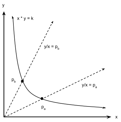
The above curve is the standard x·y=k AMM formula from V1, except we are now visualizing prices as rays extending from the origin. Any point that lies on such a ray will have a price value equivalent to any other point lying on the same line.

If we allow prices from (0, ∞), then we can have points (x, y) anywhere along the x·y=k curve. Similarly, corresponding price rays can have their direction ranging anywhere between the +x-axis and the +y-axis, with larger prices being represented by price rays leaning closer to the y-axis. However, if we restrict allowable prices to a fixed range, say [p_a, p_b], then we notice that only the part of the x·y=k curve located between the area formed by the y/x=p_a price ray and the y/x=p_b price ray may be used for exchanges. In other words, we can no longer trade Y for X when y/x=p_a is reached, and we can no longer trade X for Y when y/x=p_b is reached.

Setting a limited price range for a liquidity pool might not seem useful at first glance, but it is actually quite powerful because it means we do not need as much of token X and token Y to actually maintain the liquidity pool. Using the same graph as above, now consider the actual amount of token X and token Y needed to maintain trades between [p_a, p_b].

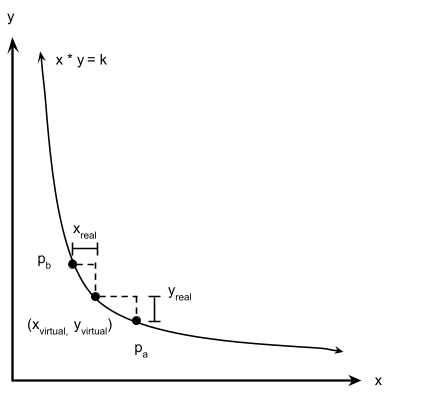
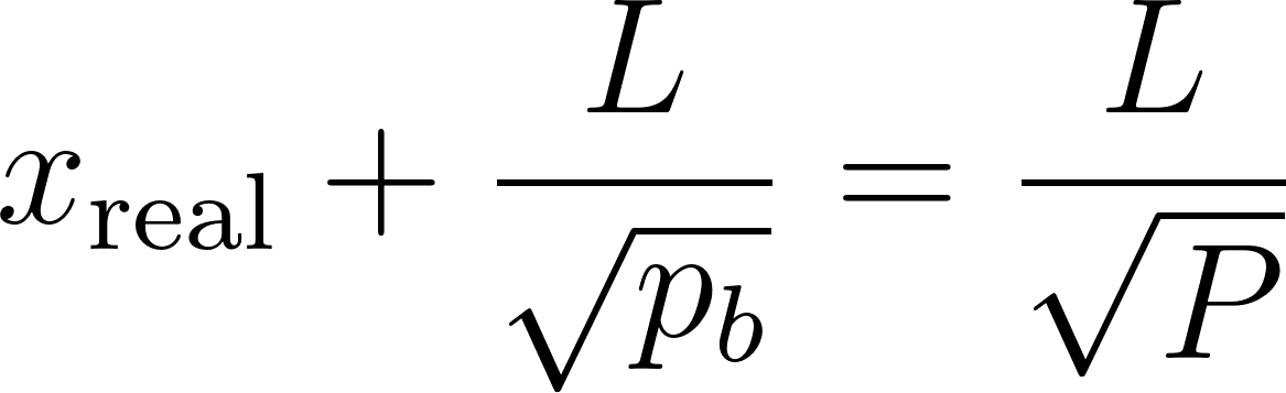
Assuming we are at the point (x_virtual, y_virtual) on the price curve, the largest amount of token X that might need to be given away in a trade is indicated by x_real in the graph, and the largest amount of token Y that may need to be traded away is indicated by y_real. Therefore we only need a total of x_real and y_real reserves to pretend that we actually have x_virtual and y_virtual reserves [3]. We are using x_real and y_real to trade on a price-limited section of the x·y=k curve.

With this concept about prices in mind, Uniswap V3 defines the liquidity, L, on a specific price range as the square root of the product of virtual reserves on that price range. In other words, for any point (x_virtual, y_virtual) on x·y=k, we have [16]

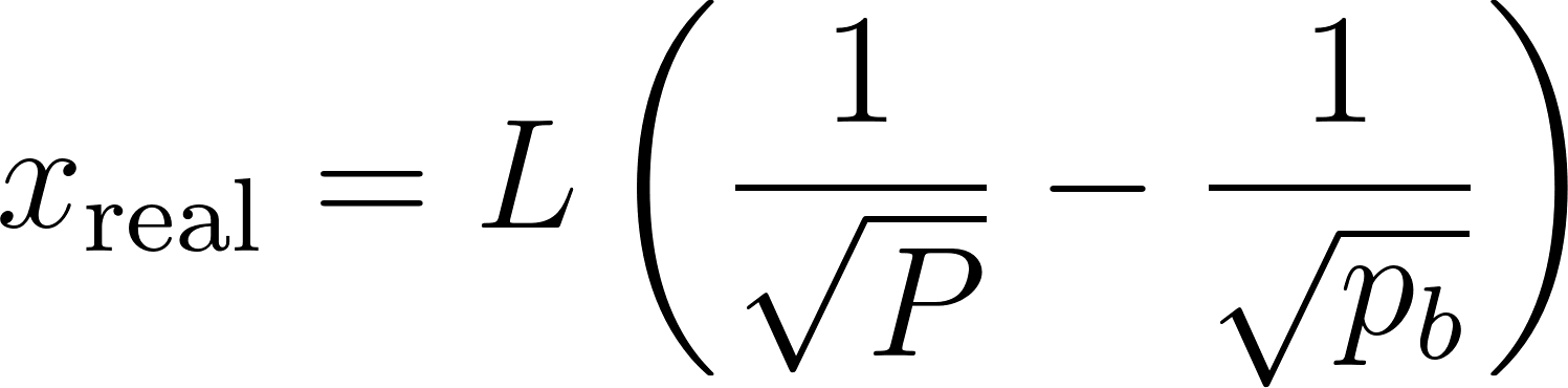
While this definition is nice, what we really want is to relate the liquidity on a price range to its real reserves. To do this, we can first think write x_virtual and y_virtual in terms of x_real, y_real, p_a, p_b, and L. See section 7.8 for a full derivation, but the gist is that we end up with equation 2.2 from the Uniswap V3 whitepaper.

So far we've learned that each price range can have its own liquidity reserves, which define its own price curve. What happens when we have a liquidity pool with multiple price ranges, each with a different liquidity reserve?

In Uniswap V3, price ranges are discretized into small segments between markers called "ticks". Each tick corresponds to a specific price, and users can only provide liquidity on a price range with starting/ending points both on a tick mark [13]. The price represented by tick i, for i = ... −2, −1, 0, 1, 2 ..., is as follows:

The price of each consecutive tick is 0.01% (1 basis point) more than the previous tick. Using the same price visualization from before, where each price is represented by a ray starting from the origin, we can visualize ticks according to the following graph:

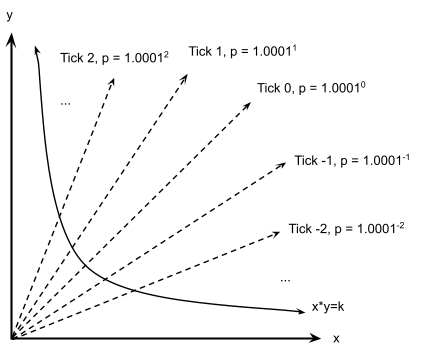
The area between two consecutive ticks is a small price range, so ticks help us discretize nearly the entire range (0, ∞) into these small price ranges (the max tick is 887272). In the above diagram, there is only a single x·y=k curve, and liquidity is set to be continuous on the entire range (0, ∞). However, ticks allow for every tick range (price range) to have its own liquidity reserves and thus its own curve! For example, varying liquidity allocation to the different price ranges could make in the liquidity pool look like the following [13]:

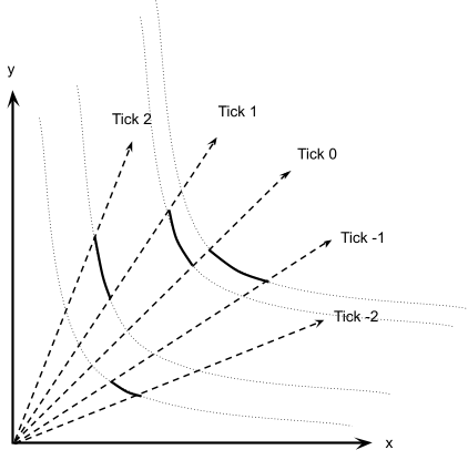
Because liquidity providers are no longer uniformly distributing their liquidity from (0, ∞), it is likely that each price range has a different total amount of liquidity, and therefore follows a different x·y=L² curve. For each curve, the region where it is inside its corresponding price range is highlighted. This region will dictate for the price range, how the price as well as x_real and y_real move during a swap. Also notice that the more liquidity L a price range has, the further out its price curve will be from the origin.

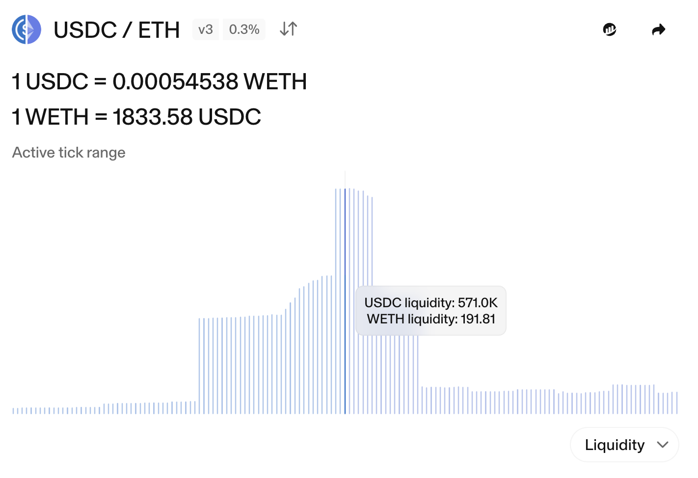
While the above graph is useful, it more frequently appears as a bar chart, with tick number on the x-axis and the amount of liquidity between two ticks represented by a corresponding bar. For example, see the USDC/ETH liquidity chart in the appendix section 7.1.

3.2 Swaps and Providing Liquidity

Given the new model of concentrated liquidity and price ticks, a natural question is how Uniswap V3 performs the basic operations of swapping tokens and providing liquidity, especially if they can span multiple tick ranges.

Starting with swaps, users will input how much of one token they want to exchange for the other type of token (e.g. some token X for some token Y). The price will start shifting along the curve of the current tick range, using up liquidity in the range until the liquidity becomes only the type of token the user wants to sell (e.g. only token X). At this point the swap will have reached the next tick, and the liquidity in the next tick range will start being exchanged as well. This continues until the swap is completely satisfied [12]. A visual representation of the price and liquidity movement during a swap is shown in the below diagram:

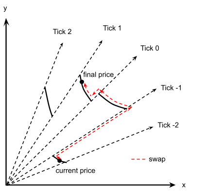
When the current price is within a tick range, it moves according to the price curve for that range. When it reaches a tick, the price remains constant, and instead the liquidity moves to match the liquidity of the new price range that is being entered. These liquidity movements when the price reaches a tick mark are also called "crossing a tick".

Going a bit further into the implementation and math behind a swap, consider a swap where a user trades y_input tokens of Y for as many tokens of X as possible. Let the current price before the swap be P and the liquidity of the current tick range be L. We need to calculate how much of the input tokens Δy the current tick range can exchange before reaching the next tick. To do this we can re-use the main formula derived in the previous section and substitute values using the range [P, p_b] to solve for x_real and y_real. See section 7.9 for a derivation.

The derivation can actually be generalized to yields two generic formulas for x-movement Δx and y-movement Δy along a price curve, based on the price movement ΔP and liquidity value L [10].

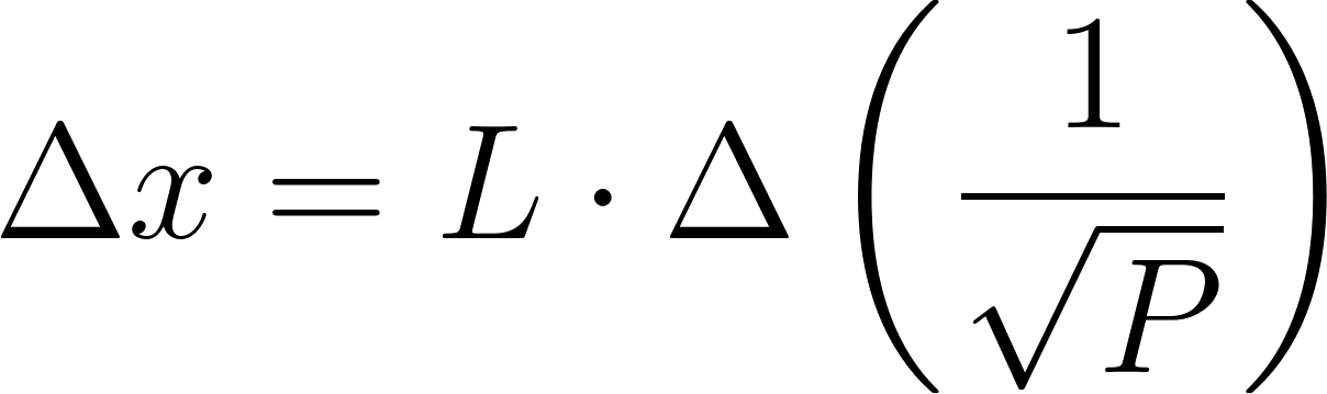
In essence, Uniswap V3 performs a swap of y_input tokens of Y as follows [12].

• It first determines ΔP to the next tick = price of the next tick − current price, with L remaining constant since we stay on the same price curve. Then it can calculate Δy.
• If Δy is greater than y_input, we can use y_input to calculate the corresponding actual price movement ΔP that is needed to use it all up, and then use that ΔP to calculate how much Δx is received.
• Otherwise if Δy is less than our y_input we first calculate how much Δx we receive from exchanging the maximum Δy in the current tick range. Then we move to the next tick and try to buy as much X as possible with now y − Δy tokens of Y.

In order for this to work, Uniswap V3 maintains a global price P (√P in actuality for optimization purposes) that is updated as we move along the price curve within a tick range. It also maintains a global liquidity L that is updated after when we cross a tick [16]. P may naturally be updated based on ΔP from the calculations above, but we have not yet discussed how Uniswap V3 updates L. To do this we must examine how liquidity is provided.

To provide liquidity, users are asked to create positions consisting of a price range [pa, pb] and a liquidity value L. pa and pb must coincide with tick marks, and they cannot be located in between two ticks. The pa value corresponds to the "lower tick" of the price range, while the pb value corresponds to the "upper tick".

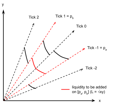
One might assume that when providing liquidity, every tick should store the liquidity reserves on the price range between itself and the next tick. Then the algorithm would update every single tick between the lower tick and upper tick, adding L to the liquidity stored for each tick range. However, Uniswap V3 uses a clever optimization of storing on each tick the change in liquidity when the price passes over it (from a lower tick). For each tick, this stored quantity is called netLiquidity [11]. Now whenever a user provides a position with an additional ΔL liquidity, Uniswap updates netLiquidity += ΔL for the position's lower tick and netLiquidity −= ΔL for the position's upper tick. netLiquidity does not need to be updated for any other tick.

When a swap happens (let's assume the price increases during this swap) and the price crosses over any tick, Uniswap adds the tick's netLiquidity to the global variable storing the current liquidity L. So when the price crosses over the lower tick of a position, the position's liquidity will be included in calculations for all tick ranges up until the upper tick [11]. After the price crosses over the position's upper tick, the position's liquidity will get subtracted from the current liquidity L, and this liquidity will not be included for future ticks that are past the upper tick.

3.3 Architectural Changes

There were several architectural changes made from v1 and v2 compared to v3. In v1 and v2, every pair of tokens was fixed to one liquidity pool with a 0.3% swap fee. This faced some issues with adaptability, especially with different market conditions. This fixed fee tier may be too high or low for certain pools. Hence in v3, multiple pools are used for each pair of tokens with differing swap fees. These pools are created by the same factory contract where three different fee tiers exist: 0.05%, 0.3% and 1% [3].

Another significant change with earlier versions is non-fungible liquidity. In v1 and v2, liquidity providers' earned fees were automatically deposited in the pool as liquidity. In v3, fees are stored on their own through the tokens collected upon swap [3]. Furthermore, liquidity provider shares in v1 and v2 were represented by ERC-20 tokens. These were the liquidity held in the pool. V3 decided to discard this idea by making liquidity positions non-fungible – using ERC-721 tokens. These changes allow the LP to choose their price range and collected fees. This gives developers more flexibility to make tools that are able to manage these positions like reinvestment logic.

In terms of similarities, Uniswap v2 and v3 are similar in the sense that they have a protocol fee that can be turned on by UNI governance. The difference is that in v3, UNI governance is more flexible when choosing the fraction of swap fees. In particular, they can choose any fraction 1/N where 4 ≤ N ≤ 10 or zero [3]. UNI governance also adds additional fee tiers and tick spacing (for price ranges). This helps ensure that the new fee tier remains consistent with the integrity of the Automated Market Maker's design. Once these parameters have been added, it is immutable and cannot be changed or removed.

In addition to these changes, Uniswap v3 also made three changes to the time-weighted average price (TWAP) oracle introduced in v2. The biggest modification is how v3 eliminates the need to manually track and store previous values of the accumulator externally. This is done through introducing checkpoints of the accumulator value into the protocol [3].

In previous versions, v2 computed the arithmetic mean TWAPs. In v3, this is replaced by using the geometric mean TWAPs [3]. Instead of finding the sum of the raw price values, the protocol now takes the log of those prices using the logarithm base 1.0001 of the price:

This is known as the tick index. The accumulator at some given time is then the cumulative sum of this tick index:

For some time period [t1, t2], we can find the time-weighted geometric mean price P_t1,t2 through the following:

If values for the log price accumulator at time t1 and t2 are represented as a1 and a2 respectively, this formula can be transformed to the following:

Here, (a_t2 − a_t1) represents the total sum of log_1.0001(P) from t1 to t2. If this is converted back to log-scale, price is found to be:

Besides price tracking, v3 also incorporates a liquidity oracle by keeping track of the accumulator of 1/L (reciprocal of liquidity over time). This is tracked through secondsPerLiquidityCumulative (spl) where external contracts can use this to distribute rewards. If a contract would like to reward some position with liquidity L from time [t0, t1], at a rate of R tokens per second, this can be written in the following:

This applies directly to Uniswap v3 as it supports concentrated liquidity where the accumulator is updated when a position is within range and the checkpoints are stored whenever a tick is crossed.

4. Uniswap V4

4.1 Overview of Hooks

Hooks in Uniswap v4 brought about big changes in decentralized exchange architecture. This was done through the introduction of external smart contracts which allowed for the customization of Automated Market Maker functionalities. Hooks themselves are external contracts that are plugged into liquidity pools. Each liquidity pool in Uniswap v4 is associated with one hook contract [6]. However, one hook contract can serve multiple pools at the same time. Hooks allow for the possibility of running custom logic at various points during the lifecycle of Uniswap's liquidity pool. This form of flexibility allows alterations in the behavior of token swaps, pool initialization, liquidity management, and other AMM logic.

Hooks work through callback functions that are triggered during various times in the lifecycle of a pool [7]. Therefore, developers can now implement custom logic before or after some event occurs within the pool. The 14 different hook callback functions are as follows [4]:

• Hooks for Initialization
  • beforeInitialize and afterInitialize: called during the initial setup and creation of liquidity pools
• Hooks for Liquidity Management
  • beforeAddLiquidity and afterAddLiquidity: called when liquidity is added to the pool
  • beforeRemoveLiquidity and afterRemoveLiquidity: called when liquidity is removed
• Hooks for Swap Operations
  • beforeSwap and afterSwap: called during token swaps
• Hooks for Donation
  • beforeDonate and afterDonate: called when tokens are donated to the liquidity pool
• Hooks for Delta
  • beforeSwapReturnDelta and afterSwapReturnDelta: called during token swap and when token deltas are returned
  • beforeLiquidityReturnDelta and afterAddLiquidityReturnDelta: called when liquidity is added and token deltas are returned

Uniswap V4 also introduces the concept of "deltas". These refer to adjustments made to the token quantity when swaps or changes in liquidity occur [7]. This concept allows developers to change the default swap behavior and apply custom trading logic like stable swap curves or dynamic fees. For example, a hook contract can return deltas that can incorporate dynamic fees in response to market conditions where real-time fee calculations are accounted for.

4.2 Hook Encoding and Deployment

Hook permissions are directly encoded into the contract's Ethereum address. In other words, it consists of bits within this address where each callback function refers to some specific bit. This means that the PoolManager, the centralized managing contract that holds the state of all the liquidity pools, scans the address before determining which callback function to make. In other words, the hook contract self-declares which of the callbacks it uses [8]. For example, the beforeSwap and afterSwap callback functions correspond to the 7th and 8th bit of the hook contract's address. Given some Ethereum address:

0x00000000000000000000000000000000000000C0

If this address is translated to binary, the result is the following:

0000 0000 0000 0000 0000 0000 0000 0000 0000 0000 0000 0000 0000 0000 0000 0000
0000 0000 0000 0000 0000 0000 0000 0000 0000 0000 0000 0000 0000 0000 0000 0000
0000 0000 1100 0000

The binary ends in 1100 0000 where the 1st to 6th bit is 0 while the seventh and eighth bit is set to 1. The PoolManager will then execute the functions where their corresponding bit is 1. If the bit is 0, that callback function is skipped [8]. The use of this encoding is important as it ensures that the addresses remain immutable upon deployment. It also prevents issues with storage by using the address as a permission bitmap. PoolManager checks a hook's capabilities by masking the address — no storage read nor delegate call — so adding a hook costs the gas of a bitwise AND. Because the address cannot be changed after deployment, liquidity providers can reason about the exact code that will run on their positions.

4.3 Pool Manager

One of the main differences between Uniswap V3 and V4 is how pools are handled: Uniswap V3 manages pools as distinct contracts while Uniswap v4 combines management of these pools into a single contract through PoolManager.sol. Five external entry points — initialize, modifyLiquidity, swap, donate, and settle — cover the full lifecycle of a pair. Each pool carries a PoolKey (addresses, fee tier, tick spacing, hooks contract) so PoolManager can locate the correct row in its storage map [9]. Because every pool shares libraries and event definitions, routers compile smaller and auditors stare at less code. For pool initialization, the following function describes how it is done in PoolManager [9]:

function initialize(PoolKey memory key, uint160 sqrtPriceX96) external
    noDelegateCall returns (int24 tick) {
    // see TickBitmap.sol for overflow conditions that can arise from tick
    // spacing being too large
    if (key.tickSpacing > MAX_TICK_SPACING)
        TickSpacingTooLarge.selector.revertWith(key.tickSpacing);
    if (key.tickSpacing < MIN_TICK_SPACING)
        TickSpacingTooSmall.selector.revertWith(key.tickSpacing);
    if (key.currency0 >= key.currency1) {
        CurrenciesOutOfOrderOrEqual.selector.revertWith(
            Currency.unwrap(key.currency0), Currency.unwrap(key.currency1)
        );
    }
    if (!key.hooks.isValidHookAddress(key.fee))
        Hooks.HookAddressNotValid.selector.revertWith(address(key.hooks));

    uint24 lpFee = key.fee.getInitialLPFee();

    key.hooks.beforeInitialize(key, sqrtPriceX96);

    PoolId id = key.toId();

    tick = _pools[id].initialize(sqrtPriceX96, lpFee);

    // event is emitted before the afterInitialize call to ensure events are
    // always emitted in order
    // emit all details of a pool key. poolkeys are not saved in storage and
    // must always be provided by the caller
    // the key's fee may be a static fee or a sentinel to denote a dynamic fee.
    emit Initialize(id, key.currency0, key.currency1, key.fee,
        key.tickSpacing, key.hooks, sqrtPriceX96, tick);

    key.hooks.afterInitialize(key, sqrtPriceX96, tick);
}

initialize() takes in a PoolKey struct and a sqrtPriceX96 variable as its parameters. The PoolKey struct shown in Appendix 7.2 involves all of the properties that make up a pool like its address, hooks, and tick spacing [9]. The sqrtPriceX96 variable represents the square root of token1's starting price in respect of token0 encoded in Uniswap's Q64.96 fixed-point format.

Several safety checks are then performed by checking if the tickSpacing is within the bounds of MAX_TICK_SPACING and MIN_TICK_SPACING. Several other validation checks are done including checking the hook address with isValidHookAddress(). If the hooks are not configured correctly, the contracts revert. After completing the validation checks, the initial liquidity provider fee (lpFee) is retrieved and beforeInitialize() is called on the hooks [9]. Initialization finally begins by calling _pools[id].initialize() which creates the state for the pool and determines what the tick index is. This tick index is responsible for determining price levels and where liquidity is placed. The tick value that is returned after this is called is the result that falls within the tick boundaries. The function continues by emitting an Initialize event with all of the information about the pool and eventually calls afterInitialize on the hook contracts [4].

To add or remove liquidity from a pool, the modifyLiquidity() function in Appendix 7.3 is called [9]. The modifyLiquidity() function takes in three parameters: key (metadata that uniquely identifies a pool), params (has the parameters for modifying liquidity), and hookData (extra data sent for hook pre and post-processing). The function begins by first generating a unique identifier for a given pool. The state of the pool is then retrieved through _getPool(id) and checked if it has been initialized through checkPoolInitialized() [17]. Before modifying the liquidity, if developers would like to inject some custom logic, beforeModifyLiquidity() is called. The function that calls pool.modifyLiquidity() to add or remove liquidity, calculates the delta through the base liquidity delta and the fees they had accrued which will eventually be considered against the balance. afterModifyLiquidity() is then called for any post-processing.

PoolManager also incorporates a swap() function in Appendix 7.4 where token swaps of two assets are involved. The method takes in PoolKey (identifying which pool through addresses), SwapParams (instructions for swapping), and hookData as its parameters [9]. The SwapParams instructions are important here as it mentions the amount that is swapped (amountSpecified), and the direction to which the swap occurs. Several checks are also done to make sure what is swapped makes sense. For instance, if the amountSpecified is set to 0, the function would revert because a zero swap is meaningless. This also helps prevent exploitation of this method by constantly calling zero swaps. The pool is then determined and checked for initialization. The beforeSwap() hook is called which enables developers to change the amount that can be swapped. After this is called, the amountToSwap result is sent to the _swap() function where the actual trade is done through pool.swap(params). The method then continues with an afterSwap() hook for any post-swap processing [18].

The donate() function in Appendix 7.5 allows the user to add assets to the liquidity pool without receiving anything in return. The method takes in PoolKey which just identifies the pool, amount0 and amount1 are the amount of token0 and token1 that are donated to the liquidity pool, and hookData [9]. To begin donation, the function gets the pool and checks for initialization. The beforeDonate() hook is called for implementing any custom logic prior to token donation. pool.donate(amount0, amount1) is called where this method adds the specified number of tokens to the pool and a delta value is returned. To ensure integrity throughout the whole system, token donations are still recorded even though the user does not receive anything in return. Finally, the afterDonate() hook is called.

To protect both the registry and external hooks from re-entrancy, v4 introduces the lock-unlock pattern. Several of these functions also use a security model called the unlock callback system which can be seen in Appendix 7.6 [7]. The onlyWhenUnlocked() modifier acts as a guard for all of the functions previously mentioned. If the PoolManager is not in an unlocked state, this will prevent it from moving forward with the function [9]. During this unlocked window, permission is granted to a caller to be able to execute some of the actions like modifying liquidity through the unlockCallback function. This helps prevent any unauthorized function from changing the state of the pool. These state-changing methods power users' batch operations with an unlock(bytes) escape hatch. Inside the hatch, they might add liquidity to pool A — each action pushes a BalanceDelta into transient storage. When control returns, PoolManager sums the per-currency deltas, verifies every pool is still solvent, and only then flips the global lock. If any delta remains unsettled, the whole transaction reverts, stopping a compromised hook dead before it can externalize losses.

4.4 Flash Accounting and Fees

In Uniswap v4, a singleton design pattern is used instead of the factory/pool pattern in the previous Uniswap protocols, allowing all pools to be managed by a single contract. However, the singleton would not matter if every hop still paid the full ERC-20 transfer cost, so v4 layers flash accounting on top of EIP-1153 transient storage [22]. EIP-1153 introduces dedicated transient storage slots that live only for the duration of a single transaction. Instead of writing to expensive permanent storage (SSTORE), hooks and internal PoolManager functions emit a struct BalanceDelta { int128 amount0; int128 amount1; } and write them to transient slots via the new TSTORE(Δslot, packedDelta) opcode. Each TSTORE costs just one gas and its data vanishes when the transaction completes [23]. Reading these deltas uses the complementary TLOAD opcode.

During an unlock session — a window in which a user can batch arbitrary swaps, liquidity adds/removals, and donations — every balance-changing call appends its delta to the transient slot for that token. When the session ends, PoolManager nets all BalanceDeltas per currency:

for each token C observed this tx {
    int256 net = ΣΔ[C];
    if (net > 0) IERC20(C).transferFrom(caller, address(this), uint(net));
    else if (net < 0) IERC20(C).transfer(caller, uint(-net));
}

So the caller settles just one ERC-20 transfer per currency, regardless of path length. A real-world benchmark posted by the Uniswap Foundation shows that a four-hop route that would have cost approximately 190 kGas in v3 now clears in approximately 110 kGas (nearly a 40% reduction) because intermediate transfer calls are netted away [22].

Inside each swap, the protocol first removes the liquidity provider fee:

where lpFee may have been dynamically set by a hook seconds earlier. Of that fee, a fraction 1/N (4 ≤ N ≤ 10) is siphoned into the protocol-fee vault if governance has toggled the switch [24]. Both liquidity pool and protocol fee accrue in-pool as owed amounts rather than being reinvested, thus breaking the auto-compounding of v2/v3 and making it trivial for liquidity pool management contracts to harvest and redeploy custom logic.

AfterSwap hooks can adjust fees again by returning their own BalanceDelta. Imagine a volatility-sensitive hook that widens the spread when five-minute realized variance exceeds a threshold:

function afterSwap(...) returns (BalanceDelta swapΔ, BalanceDelta hookΔ) {
    if (volatility() > σ*) {
        // rebate 2 bp to taker, collect 3 bp to LPs
        hookΔ = BalanceDelta({amount0: int128(-rebate0), amount1: int128(-rebate1)});
        swapΔ.amount0 += rebate0;
        swapΔ.amount1 += rebate1;
    }
}

Because hook deltas merge with swap deltas in transient storage, the caller still settles only once per currency.

The last piece is fee withdrawal. Liquidity providers call modifyLiquidity with liquidityDelta = 0 to trigger an internal _collectFee() that burns owed amounts off the pool's fee-growth accumulator and pushes them to the LP's wallet.

Protocol-fee sweep is an owner-only action on the vault, gated by a 7-day timelock baked into the governance module [25]. Both flows are plain ERC-20 transfers, so they inherit all the gas gain from flash accounting.

4.5 Some Instances of Hooks & Their Implementations

Uniswap v4 introduces a flexible, hook-based architecture that enables advanced AMM features — such as TWAP orders, volatility oracles, limit orders, and dynamic fees — to be implemented without modifying the core protocol. This significantly expands the design space compared to Uniswap v3.

These hooks are often grouped into what developers call the "big four" categories. The first category is liquidity profitability, which includes mechanisms like dynamic fees, rehypothecation, and liquidity auctions. These features aim to improve the earnings potential for liquidity providers by adapting fees to market conditions or optimizing capital efficiency. The second category is liquidity depth, which encompasses tools for strengthening the depth and stability of liquidity in pools. Examples include long-term liquidity incentives, just-in-time (JIT) liquidity provisioning, and on-chain limit orders. These mechanisms help ensure that liquidity is both available and responsive to trading needs, allowing for support of larger volume trades.

The third category is asset class support, enabling pools to accommodate a broader range of token types. This includes real-world assets (RWAs) that may require compliance constraints, liquid staking tokens that benefit from custom pricing curves or liquidity management tricks, and rebasing tokens that can be automatically wrapped or unwrapped. Governance tokens can be integrated to allow voting with the LP's underlying assets, and even memecoins can benefit from hooks that tailor volatility exposure or manage incentives. The final category, sometimes referred to as public goods, is a catch-all for features that improve market infrastructure more broadly. This includes alternative trading order types like TWAMM and limit orders, as well as the integration of various oracle types — manipulation-resistant price feeds, volume oracles, and volatility oracles. For instance, a lending protocol could use a volume oracle to adjust its parameters based on pool depth, offering more favorable terms when liquidity is deep. Public goods also broadly support diverse asset classes and tokenomic models, enhancing composability across the DeFi ecosystem.

In the following subsections, we dive deeper into some specific instances of hooks: TWAMM, dynamic fee, limit order and stop loss hooks.

4.5.1 TWAMM

The Time-Weighted-Average Market Maker (TWAMM) [32] works by breaking long-term orders into infinitely many infinitely small pieces and executing them against an embedded constant-product AMM smoothly over time [28]. An implementation example of TWAMM can be found in the github repo [29], and for a more rigorous derivation for the outcome of virtual trades in TWAMM, refer to section 7.7 in the Appendix of this report.

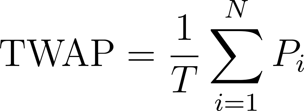
This mechanism essentially replicates the traditional finance concept of a Time-Weighted Average Price (TWAP) strategy, adapted for on-chain execution. In traditional markets, TWAP is used to execute large orders by splitting them into smaller, evenly spaced trades over a set time period. The idea is that by trading consistently over time, the trader ends up transacting at the average market price during that window. This time-neutral approach aims to minimize market impact and reduce the risk of signaling large directional intent, thereby achieving a "fair" execution price without introducing unnecessary volatility.

Consider the following concrete example: suppose that Alice wants to buy 100 million USDC worth of ETH in the next 8 hours, or about 2000 blocks. The long-term order she enters allows her to buy on average 50000 USDC per block. Since we don't know which miners will process the transactions these orders must be visible to everyone.

Suppose that in the order pool we have Bob who wants to sell 500 ETH for USDC over the next 5000 blocks, or 0.1 ETH per block, AND we have Charlie who wants to sell 100 ETH for USDC over the next 2000 blocks, or 0.05 ETH per block. Until Charlie's order expires, Bob and Charlie's orders would be grouped together and live in a pool. Bob would earn 66% of the profits made from trading ETH in the pool, and Charlie would earn 33%.

The TWAMM (Time-Weighted Average Market Maker) models large trades by dividing them into an infinite number of infinitesimal sub-orders that are executed continuously over time. This idealized splitting results in perfectly smooth price trajectories, which aligns well with the assumptions underlying TWAP execution — namely, that large-volume trades can be spread out evenly to minimize price impact. Crucially, this formulation allows the entire trade's effect on the pool to be computed analytically in a single step, without simulating each sub-order individually. While this model works well in the case of a single large trader, extending it to handle multiple simultaneous large trades — especially in opposing directions — introduces additional complexity. In practice, such scenarios are less common and may require more sophisticated virtual execution logic or approximation methods.

The buy and sell orders are executed in turn, in a back-to-back fashion. Since Alice is buying more than the pool is selling the price of ETH will go up in the current pool, and arbitrageurs could buy ethereum from other pools with a cheaper price and sell it in the pool where Alice is located, meeting the demand for ETH and gaining a profit.

Since Alice, Bob and Charlie are not pushing for time to execute their orders, the outsiders can infer that there is less adverse selection at play and thus offer to trade at lower fees.

In implementing this, we make use of the following key ideas: lazy evaluation and order pooling. Since the virtual suborders are treated as if they happened in between blocks, the gas efficient way for execution is only to evaluate the effect of a virtual trade when necessary and not exactly by the time that it occurs. This lazy evaluation approach means that whenever a user interacts with the TWAMM, it retroactively calculates the effect of all the virtual trades that took place since the last interaction. When we have a few long-term orders in the same direction, the orders are pooled together before being split into virtual trades. Notice that order pooling and lazy evaluation in conjunction could mean that order expiry within a given pool can happen on any date or can continuously occur on many separate dates, which forces the orders in the pool to split up, resulting in a lack of efficiency. This is why the expiry dates of orders are required to occur every 250 blocks or roughly once per hour.

Virtual trades in a TWAMM are resistant to sandwich attacks because they are not discrete transactions submitted to the mempool, but rather continuous flows that are executed analytically between blocks. Instead of executing each small trade in real-time, the TWAMM computes the net effect of all virtual trades that should have occurred since the last interaction with the pool. This means there is no exact timestamp or transaction that an attacker can front-run or back-run in the traditional sense.

For an attacker to sandwich a virtual trade, they would need to predict and precisely control the execution window across block boundaries — inserting a front-running trade at the very end of one block, and then a back-running trade at the very start of the next. Even then, the effect would be diluted, because TWAMMs calculate trades as an aggregate over time, and the impact of any one attack window is minimal. The attacker would also need to pay more gas, take on more risk, and compete with MEV searchers for block timing, making the attack less economically viable.

4.5.2 Dynamic-Fee Hook

Uniswap v4's dynamic fee system enables advanced behavior through hooks. For example, pools can stabilize soft pegs by charging lower fees on trades that bring the price closer to the peg, and higher fees on trades that push it away. Directional fees can also simulate dual pricing, where buy and sell trades have different effective prices. Since liquidity providers may accumulate the underperforming token in volatile markets, custom hooks can be designed to periodically buy out this token, helping to rebalance positions. Additionally, hooks can implement MEV-aware logic: by recognizing patterns consistent with sandwich attacks or frontrunning, they can dynamically increase fees on high-risk swaps, effectively acting as a 'MEV tax' and discouraging predatory behavior [26].

Dynamic-fee hooks in Uniswap v4 allow swap fees to adapt to real-time market conditions. A notable use case is volatility-aware fee adjustment: by sampling an on-chain realized-volatility oracle at each swap, the hook can increase LP fees during periods of market turbulence [27]. This mitigates impermanent loss and discourages MEV strategies like sandwich attacks. In contrast, Uniswap v3 and static-fee v4 pools use fixed fee tiers set at deployment (e.g., 0.05%, 0.3%, 1%), which cannot respond to shifts in volatility. Dynamic-fee hooks offer a flexible alternative that better aligns fees with market risk.

In practice, the hook's beforeSwap callback reads the on-chain volatility in basis points — so a value of 250 represents 2.5% volatility — and applies a simple formula: a 0.30% base fee plus an additional 0.05% for each full percentage point of volatility. The core logic is succinct:

function beforeSwap(
    PoolKey memory key,
    SwapParams memory params,
    bytes calldata
)
    external view override
    returns (int256 amountToSwap, BalanceDelta hookDelta, uint24 lpFeeOverride)
{
    uint24 volBp = IVolatilityOracle(key.hooks).vol30d(key.currency0, key.currency1);
    // Base 30 bp + 5 bp per full percent of realized vol
    lpFeeOverride = 30 + (5 * volBp) / 100;
    return (params.amountSpecified, BalanceDeltaLibrary.ZERO_DELTA, lpFeeOverride);
}

By overriding lpFeeOverride, the hook compensates LPs during turbulent periods without affecting long-term pool state.

4.5.3 Limit Order Hook

Decentralized exchanges have struggled to offer trustless limit orders without bloating gas costs. The Limit-Order Hook addresses this by moving the order matching process off-chain (usually to a decentralized order-book service) while retaining trust-minimized execution on-chain through the beforeSwap callback [30][33]. When a user submits a signed limit order, it's stored off-chain and remains inactive until the market conditions meet the user's specified price. At that point, the hook automatically executes the trade atomically within the Uniswap pool.

Upon each swap attempt, the hook checks whether there is a matching limit order in the off-chain book that satisfies the swap's price parameters. If a match is found, the hook allows the swap up to the limit order's remaining amount. This ensures limit orders are executed only when prices are favorable, and otherwise the transaction is deferred.

function beforeSwap(
    PoolKey memory key,
    SwapParams memory params,
    bytes calldata
)
    external
    override
    returns (int256 amountToSwap, BalanceDelta hookDelta, uint24 lpFeeOverride)
{
    bytes32 poolId = keccak256(abi.encode(key.currency0, key.currency1, key.fee));
    LimitOrder memory top = book.getTopOrder(poolId);
    uint256 price = getPoolPrice(key);

    // If a buy order's limit price >= current price, fill up to remaining amount
    if (params.zeroForOne && top.price >= price) {
        uint256 fill = top.amount - top.filled;
        book.fillOrder(top.id, fill);
        return (int256(fill), BalanceDeltaLibrary.ZERO_DELTA, params.lpFee);
    }
    return (params.amountSpecified, BalanceDeltaLibrary.ZERO_DELTA, params.lpFee);
}

This design minimizes on-chain state changes (only the filled portion triggers a book update) and preserves Uniswap's atomicity; either the limit order executes in full within the swap transaction, or the entire swap reverts, guaranteeing trust-minimized execution with negligible extra gas overhead [31].

4.5.4 Stop-loss Hook

In highly dynamic markets, LPs and takers often race the risk of severe losses if prices move sharply beyond their anticipated range. The Stop-Loss Hook provides an on-chain "circuit-breaker" by embedding stop-loss orders directly into Uniswap v4's PoolManager workflow, eliminating reliance on external keepers and ensuring guaranteed execution [34].

A hedger initiates a stop-loss order by calling the hook's order-creation function and specifying a trigger tick and position size. Upon creation, the hook mints an ERC-1155 receipt token to the user, representing a claim on future execution proceeds. This receipt can be freely transferred or used as collateral, enabling composability with other DeFi protocols.

As normal swaps execute through PoolManager, the hook's afterSwap callback fires after every trade. It scans all active orders, compares each order's trigger tick to the current pool tick index and if a stop-loss condition is met, performs on-chain depth checks to ensure sufficient liquidity and acceptable slippage. Once the order has been successfully executed, the hook marks the order as such and records the proceeds in its internal ledger.

function afterSwap(
    PoolKey memory key,
    SwapParams memory,
    BalanceDelta swapΔ,
    bytes calldata,
    BeforeSwapDelta memory
)
    external override
    returns (BalanceDelta, BalanceDelta hookΔ)
{
    int24 tick = key.hooks.getCurrentTick(key);
    for (uint i = 0; i < activeOrders.length; i++) {
        Order storage ord = activeOrders[i];
        if (!ord.executed && tick <= ord.triggerTick) {
            uint128 proceeds = executeSwap(ord.amount);
            ord.executed = true;
            orderProceeds[ord.id] = proceeds;
        }
    }
    return (swapΔ, BalanceDeltaLibrary.ZERO_DELTA);
}

Once the swap executes, any holder of the corresponding ERC-1155 receipt may call redeem(orderId) to burn the receipt and withdraw the recorded proceeds. This entire lifecycle — from order creation through execution to redemption — occurs on-chain, trustlessly and atomically.

5. Conclusion

This paper has explored the trajectory of Uniswap from its inception as a simple constant-product AMM in V1 to its current incarnation in V4 as a flexible and extensible protocol layer. We examined how each major version introduced architectural innovations that expanded both usability and expressivity: V1's ETH-centric pools and simplicity, V2's support for ERC-20 pairs and on-chain oracles, V3's concentrated liquidity and fine-grained fee customization, and finally, V4's introduction of hooks and flash accounting, which opens the door to truly programmable AMMs.

The hook system in Uniswap V4 represents a paradigm shift. No longer limited to static fee models or liquidity logic, developers can now build pools that respond dynamically to market conditions, manage risk more intelligently, and support a broader array of token types and financial behaviors — from TWAMMs and limit orders to automated liquidity management and volatility-aware fee structures. These innovations not only benefit liquidity providers through better capital efficiency and risk mitigation but also improve execution quality and user experience for traders.

Looking forward, Uniswap's new architecture suggests a future where DEXes function more like programmable platforms than fixed protocols. We may see the rise of "meta-pools" tailored to specific asset classes, new forms of incentive alignment through governance-aware LP tokens, and even the integration of real-world financial primitives via compliance-aware hooks. Furthermore, the composability of hooks opens up the possibility of layering AMMs with lending, staking, or insurance primitives — all within a single atomic transaction. As the ecosystem of Uniswap hooks matures, it has the potential to serve not just as a trading venue but as a foundation for the next generation of on-chain financial infrastructure.

6. References

1. Zhang, Y., Chen, X., & Park, D. (2018, October). Formal Specification of Constant Product (x*y=k) Market Maker Model and Implementation. Github. link
2. Adams, H., Zinsmeister, N., & Robinson, D. (2020, March). Uniswap v2 Core. Uniswap. link
3. Adams, H., Zinsmeister, N., Salem, M., Keefer, R., & Robinson, D. (2021, March). Uniswap v3 Core. Uniswap. link
4. Adams, H., Salem, M., Zinsmeister, N., Reynolds, S., Adams, A., Pote, W., Toda, M., Henshaw, A., Williams, E., & Robinson, D. (2024, August). Uniswap v4 Core. Uniswap. link
5. Adams, H. (2023, June 13). Our Vision for Uniswap v4. Uniswap Blog. link
6. Hooks. (n.d.). Uniswap Docs. link
7. Di Siena, G. (2024, November 6). Uniswap V4 vs V3: Architectural Changes and Technical Innovations with Code Examples. Cyfrin. link
8. Uniswap. (n.d.). Hook Deployment. Uniswap Docs. link
9. Uniswap. (2024). PoolManager.sol. Uniswap/v4-core. Github. link
10. Jeiwan. (2023). Uniswap V3 Development Book. Github. link
11. adshao. (2022). Deep Dive into Uniswap v3 Whitepaper. Github. link
12. Boogerwooger, S. (n.d.). Uniswap V3 ticks - dive into concentrated liquidity. MixBytes. link
13. Team Rareskills. (2025, January 17). Introducing ticks in Uniswap V3. RareSkills. link
14. Team Rareskills. (2024, December 23). How Concentrated Liquidity in Uniswap V3 Works. RareSkills. link
15. Team Rareskills. (2025, April 25). Uniswap V3 Factory and the Relationship Between Tick Spacing and Fees. RareSkills. link
16. Elsts, A. (2021, September 30). Liquidity Math in Uniswap v3. Github. link
17. docs.uniswap.org/contracts/v4/quickstart/manage-liquidity/increase-liquidity
18. docs.uniswap.org/contracts/v4/guides/swap-routing
19. The Uniswap V1 Smart Contracts. (n.d.). Uniswap Docs. link
20. The Uniswap V2 Smart Contracts. (n.d.). Uniswap Docs. link
21. Binance Academy. (2020, October 19). Impermanent Loss Explained. Binance. link
22. Uniswap Labs. (n.d.). Flash accounting. In Uniswap v4 concepts documentation. link
23. Uniswap Labs. (n.d.). TransientStateLibrary. In Uniswap v4 technical reference. link
24. Uniswap Labs. (n.d.). Custom accounting. In Uniswap v4 guides. link
25. JanBuidl. (2024, July 29). Uniswap V4 — Code Analysis. Block Magnates. link
26. Umbrella Research. (2024, January 4). Uniswap v4 hooks guide (II): Dynamic fees hook. Medium. link
27. PancakeSwap. (n.d.). Dynamic fee hook. PancakeSwap Documentation. link
28. Paradigm. (2021). TWAMM. Retrieved May 8th, 2025, from link
29. 0xnirlin. (2024, Oct 27th). TWAMM on Uniswap v4. link
30. Gee, J. (2023, November 21). Uniswap V4 limit order hook part 1: Smart contract source code analysis. Tokamak Network. link
31. Eugenio. (n.d.). limit-order-hooks [Computer software]. GitHub. link
32. Uniswap labs. (2023, August 24th). Uniswap v4 TWAMM Hook. Uniswap Blog. link
33. Uniswap Labs. (n.d.). LimitOrder.sol [Solidity source code]. GitHub. link
34. saucepoint. (n.d.). v4-stoploss [Solidity source code]. GitHub. link

7. Appendix

7.1 Uniswap V3 USDC/ETH Liquidity Diagram

7.2 PoolKey struct

struct PoolKey {
    /// @notice The lower currency of the pool, sorted numerically
    Currency currency0;
    /// @notice The higher currency of the pool, sorted numerically
    Currency currency1;
    /// @notice The pool LP fee, capped at 1_000_000. If the highest bit is 1, the
    /// pool has a dynamic fee and must be exactly equal to 0x800000
    uint24 fee;
    /// @notice Ticks that involve positions must be a multiple of tick spacing
    int24 tickSpacing;
    /// @notice The hooks of the pool
    IHooks hooks;
}

Ref: github.com/Uniswap/v4-core/.../PoolKey.sol

7.3 modifyLiquidity() function

function modifyLiquidity(PoolKey memory key, ModifyLiquidityParams memory params, bytes calldata hookData)
    external
    onlyWhenUnlocked
    noDelegateCall
    returns (BalanceDelta callerDelta, BalanceDelta feesAccrued)
{
    PoolId id = key.toId();
    {
        Pool.State storage pool = _getPool(id);
        pool.checkPoolInitialized();

        key.hooks.beforeModifyLiquidity(key, params, hookData);

        BalanceDelta principalDelta;
        (principalDelta, feesAccrued) = pool.modifyLiquidity(
            Pool.ModifyLiquidityParams({
                owner: msg.sender,
                tickLower: params.tickLower,
                tickUpper: params.tickUpper,
                liquidityDelta: params.liquidityDelta.toInt128(),
                tickSpacing: key.tickSpacing,
                salt: params.salt
            })
        );

        // fee delta and principal delta are both accrued to the caller
        callerDelta = principalDelta + feesAccrued;
    }

    // event is emitted before the afterModifyLiquidity call to ensure events
    // are always emitted in order
    emit ModifyLiquidity(id, msg.sender, params.tickLower, params.tickUpper,
        params.liquidityDelta, params.salt);

    BalanceDelta hookDelta;
    (callerDelta, hookDelta) = key.hooks.afterModifyLiquidity(key, params,
        callerDelta, feesAccrued, hookData);

    // if the hook doesn't have the flag to be able to return deltas,
    // hookDelta will always be 0
    if (hookDelta != BalanceDeltaLibrary.ZERO_DELTA)
        _accountPoolBalanceDelta(key, hookDelta, address(key.hooks));

    _accountPoolBalanceDelta(key, callerDelta, msg.sender);
}

Ref: github.com/Uniswap/v4-core/.../PoolManager.sol

7.4 swap() function

function swap(PoolKey memory key, SwapParams memory params, bytes calldata hookData)
    external
    onlyWhenUnlocked
    noDelegateCall
    returns (BalanceDelta swapDelta)
{
    if (params.amountSpecified == 0)
        SwapAmountCannotBeZero.selector.revertWith();
    PoolId id = key.toId();
    Pool.State storage pool = _getPool(id);
    pool.checkPoolInitialized();

    BeforeSwapDelta beforeSwapDelta;
    {
        int256 amountToSwap;
        uint24 lpFeeOverride;
        (amountToSwap, beforeSwapDelta, lpFeeOverride) =
            key.hooks.beforeSwap(key, params, hookData);

        // execute swap, account protocol fees, and emit swap event
        // _swap is needed to avoid stack too deep error
        swapDelta = _swap(
            pool,
            id,
            Pool.SwapParams({
                tickSpacing: key.tickSpacing,
                zeroForOne: params.zeroForOne,
                amountSpecified: amountToSwap,
                sqrtPriceLimitX96: params.sqrtPriceLimitX96,
                lpFeeOverride: lpFeeOverride
            }),
            params.zeroForOne ? key.currency0 : key.currency1 // input token
        );
    }

    BalanceDelta hookDelta;
    (swapDelta, hookDelta) = key.hooks.afterSwap(key, params, swapDelta,
        hookData, beforeSwapDelta);

    // if the hook doesn't have the flag to be able to return deltas,
    // hookDelta will always be 0
    if (hookDelta != BalanceDeltaLibrary.ZERO_DELTA)
        _accountPoolBalanceDelta(key, hookDelta, address(key.hooks));

    _accountPoolBalanceDelta(key, swapDelta, msg.sender);
}

Ref: github.com/Uniswap/v4-core/.../PoolManager.sol

7.5 donate() function

function donate(PoolKey memory key, uint256 amount0, uint256 amount1, bytes calldata hookData)
    external
    onlyWhenUnlocked
    noDelegateCall
    returns (BalanceDelta delta)
{
    PoolId poolId = key.toId();
    Pool.State storage pool = _getPool(poolId);
    pool.checkPoolInitialized();

    key.hooks.beforeDonate(key, amount0, amount1, hookData);

    delta = pool.donate(amount0, amount1);

    _accountPoolBalanceDelta(key, delta, msg.sender);

    // event is emitted before the afterDonate call to ensure events are
    // always emitted in order
    emit Donate(poolId, msg.sender, amount0, amount1);

    key.hooks.afterDonate(key, amount0, amount1, hookData);
}

Ref: github.com/Uniswap/v4-core/.../PoolManager.sol

7.6 onlyWhenUnlocked() modifier and unlock() function

modifier onlyWhenUnlocked() {
    if (!Lock.isUnlocked()) ManagerLocked.selector.revertWith();
    _;
}

constructor(address initialOwner) ProtocolFees(initialOwner) {}

/// @inheritdoc IPoolManager
function unlock(bytes calldata data) external override returns (bytes memory result) {
    if (Lock.isUnlocked()) AlreadyUnlocked.selector.revertWith();

    Lock.unlock();

    // the caller does everything in this callback, including paying what
    // they owe via calls to settle
    result = IUnlockCallback(msg.sender).unlockCallback(data);

    if (NonzeroDeltaCount.read() != 0)
        CurrencyNotSettled.selector.revertWith();
    Lock.lock();
}

Ref: github.com/Uniswap/v4-core/.../PoolManager.sol

7.7 Mathematical Derivations for Outcomes of Virtual Trades

On a mathematical level, virtual trades work as follows: Assume it has been t blocks since the TWAMM last executed any virtual trades, assume that pool selling X was selling x_rate over the entire duration, and pool selling Y was selling y_rate over the duration. Then the total amount of x sold is t · x_rate = x_in, total amount of y sold is t · y_rate = y_in. Suppose that at the start of the time period the reserves are x_ammStart and y_ammStart respectively.

The constant product formula means that we have:

The differential equation governing the swap is:

Define a new variable

Then

Let δ = 2√(x_iny_in) / √k, then the final solution is:

Where c is:

The amount of Y that ends up in the pool selling X is basically everything that does not end up in the AMM:

And we have a similar relation for the amount of X that ends up in the pool selling Y:

7.8 Derivation of the Relationship Between Real Reserves and Liquidity on a Price Range

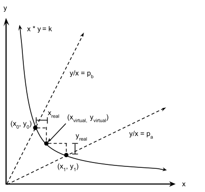
Consider the two points (x0, y0) and (x1, y1) in the above graph. The first one is where the curve x·y=L² intersects with the ray y/x=p_b. Solve this set of equations for x, and we get

Similarly, notice that (x1, y1) is the intersection of the curve x·y=L² with the ray y/x=p_a. Solve for y, and we get

Because x_virtual = x0 + x_real and y_virtual = y1 + y_real, we have

Plug into x_virtual · y_virtual = L², we end up with the equation 2.2 from the Uniswap V3 whitepaper.

7.9 Derivation of Formulas for Calculating Movement of Reserves Along a Price Curve in Uniswap V3

Solving for y_real when we are at price p_b,

Solving for x_real when we are at price P,